Bayes’ Theorem was discovered by The Reverend Thomas Bayes and was presented in his work “An Essay towards solving a Problem in the Doctrine of Chances” which was published in 1763, two years after his death. (His friend Richard Price saw to its publication.)

The theorem is foundational in the theory of probability and is widely used in philosophy of science and epistemology.

The basic idea

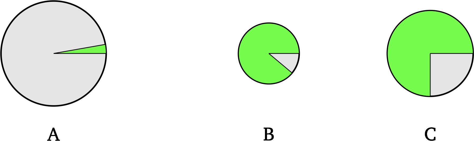
Here’s a simple scenario that brings out the basic idea. Suppose that someone has randomly chosen a specific green dot in one of these circles. You will win $1,000 if you guess correctly which of these circles contains that dot. Which circle should you choose?

You probably chose circle C. Good!

• Why not A? It’s the biggest circle. Yes, but the area of it that’s green isn’t very big.

• Why not B? It’s the circle with the greatest proportion of green. Yes but it’s smaller than C, enough so that its green area is smaller than C’s. And it’s green area that matters to the decision.

Hopefully, this reasoning convinces you. You might even think it’s obvious. It is obvious, in this simple form. But stating the principle behind this reasoning isn’t trivial. Bayes’ Theorem is the mathematical statement of that principle. We’ll work our way towards that statement. Then we will see how powerful it is when it’s applied—especially when it’s applied repeatedly.

A somewhat real-life example

Let’s go through a more real-life example, depicting it in the same circles-and-green style, and applying the same reasoning. This will be a warmup to talking about “probabilities.”

Here is some background information about Horrible Disease X:

1% of people have Horrible Disease X. There is a screening test, which is pretty reliable. But—like all screening tests—it’s not perfect. Sometimes it gives a false positive: it says you have X when you don’t. Sometimes it gives a false negative: it says you don’t have X, but you do. The rate of false positives is 10% and the rate of false negatives is 10%. (Of course, those two rates don’t have to be the same. I’m setting them to be the same just to make them easier to remember.)

Let’s suppose that you know all this background information. Then, you go to get the screening test. It comes back positive. Yikes! But you’re wondering what this actually tells you about your chance of having X. How can you think this through? What conclusion should you draw?

I strongly suggest that you pause to think this through, before going on. It doesn’t matter if you get it right. Just making the effort will improve your understanding of the correct reasoning.

We can represent the background information as follows. We have two circles. The “Don’t have X” circle is 99 times the size of the “Have X” circle. Green means someone got a positive result on their test. Of the people who have X, 90% get this result. Of the people who don’t have X, 10% get this result.

When you took the test, you got a positive result. In our diagram we represented this with green. Which of those circles are you likely to be in? In this scenario it’s the “Don’t have X” circle. You’re far more likely to be in that circle than you are to be in the “Have X” circle. Whew!

How could that be though, if your test is 90% accurate? What happened? It’s this: the test’s accuracy matters less than the huge difference in numbers between those with, and those without, disease X.

The right answer is obvious one you draw the pictures properly. But without the pictures, it’s easy to focus only on the accuracy numbers, neglecting to take into account the background likelihoods. Studies have found that even trained physicians have trouble handling these questions properly. (See for example “Probabilistic reasoning in clinical medicine: Problems and opportunities”.) It seems that we are not naturally suited to Bayesian reasoning, despite its soundness.

A preliminary calculation

We can do better than just saying that it’s “far more likely” that someone with a positive test result does not have disease X. As you should expect, we can quantify this. What we need to quantify is the portion of the green area that is in the “Have X” circle, and the portion that is in the “Don’t have X” circle, then calculate what the former is, as a percentage of all the green area. Addition and division is all this involves.

Let’s write down the background information. This is what you know before you get your test result.

To get our answer we first need to figure out the total size of the green area. There’s the bit in the small circle, plus the bit in the big circle. 90% of the size 1 circle is 0.9, and 10% of the size 99 circle is 9.9. So the total green area is 0.9 + 9.9 = 10.8.

Of that 10.8 “positive test result” area, 0.9 is in the “Have X” circle. We convert that to a percentage as follows.

$$\frac{0.9}{10.8} \times 100 = 8.3333\%$$

So, only about 8% of the people who get a positive test result are in the “Have X” circle. We have quantified what the pictures showed us.

Probabilities

The reason we need to start talking about probabilities is that they enforce a certain structure on our thinking. So far, I’ve been loose and sloppy. How?

Go back to our circles. Their relative sizes indicate the relative likelihood of their labelled conditions obtaining: it is 99 times more likely that someone doesn’t have X, than that they do have X. Now, we took for granted that those are the only two options in play. That’s an assumption that we used, but the circles themselves don’t depict that. Someone could have asked, “Why isn’t there a third circle?” and we couldn’t point to the circles in order to say why. Our answer would have to be based on the fact that you either have, or don’t have, X, and there’s no third possibility. That’s something that we know, and it does explain why there wasn’t a third circle. But it’s not something that the two circles themselves indicate.

My diagram, in other words, relied on an unspoken assumption. The assumption was that the total area of all the circles takes into account all the possibilities we’re considering. The size of a circle has a meaning only in relation to the “size” of all those possibilities. In one diagram, a size-99 circle might mean “This is very likely to happen” but in another diagram, a size-99 circle might mean “This is very unlikely to happen.” It all depends on the total space of possibilities that we’re depicting.

What we need, clearly, is a way to state these likelihoods in a self-standing way, without relying on unspoken assumptions. The language of probabilities gives us the standard way to do this.

The concept of probability

Probabilities are always thought of as numbers between 0 and 1. That’s inclusive: something having probability 0 means it’s certainly false (e.g. 1=0), and something having probability 1 means it’s certainly true (e.g. 2+2=4). We write “$Pr(p)$” to mean, “the probability that $p$,” where $p$ is some statement. $Pr(p)$ is the probability that that statement is true. (The letters “$p$” and “$q$” are used in place of statements, just like we use “$x$” and “$y$” in place of numbers in mathematics.)

We write “the conditional probability that $p$, given that $q$” as $Pr(p\ |\ q)$.

Redoing our problem using probabilities

We can now state our background information, using the language of probabilities. Here it is.

$$\begin{array}{lll} Pr(\textrm{you have X}) & = & 0.01 \\ Pr(\textrm{you get a positive result} \ | \ \textrm{you have X}) & = & 0.9 \\ Pr(\textrm{you don't have X}) & = & 0.99 \\ Pr(\textrm{you get a positive result} \ | \ \textrm{you don't have X}) & = & 0.1 \\ \end{array}$$

Let’s abbreviate things to make the reading easier:

$$\begin{array}{lll} Pr(X) & = & 0.01 \\ Pr(positive \ | \ X) & = & 0.9 \\ Pr(not\ X) & = & 0.99 \\ Pr(positive \ | \ not\ X) & = & 0.1 \\ \end{array}$$

We want to know this:

$$\begin{array}{lll} Pr(X \ | \ positive) & = & ??? \\ \end{array}$$

How can we use the first four probabilities to calculate this? Same as before. I’ll restate the calculation we did, then state it in terms of probabilities.

$$\begin{array}{ll} & \frac{\textrm{\% of small circle that's green} \ \times\ \textrm{Size of small circle}}{(\textrm{\% of small circle that's green} \ \times\ \textrm{Size of small circle})\ +\ (\textrm{\% of big circle that's green} \ \times\ \textrm{Size of big circle})} \\ & \\ = & \frac{90\% \ \times\ 1}{(90\% \ \times\ 1)\ +\ (10\% \ \times\ 99)} \\ & \\ = & \frac{0.9}{0.9 + 9.9} \ = \ \frac{0.9}{10.8} \ = \ 0.083 \ = \ 8.3\%\\ \end{array}$$

Here’s the same thing, restated in terms of probabilities:

$$\begin{array}{ll} & \frac{Pr(positive\ |\ X) \ \times \ Pr(X)} {(Pr(positive\ |\ X) \ \times \ Pr(X)) \ + \ (Pr(positive\ |\ not\ X) \ \times \ Pr(not\ X))} \\ \\ = & \frac{0.9 \ \times \ 0.01}{(0.9 \ \times \ 0.01 ) \ + \ (0.1 \ \times \ 0.99 )} \\ \\ = & \frac{0.009}{0.009 \ + \ 0.099} \ = \ \frac{0.009}{0.108} \ = \ 0.0833 \\ \end{array}$$

That final number is the value of $Pr(X\ |\ positive)$. We’re now able to state Bayes’ Theorem as it applies in this case:

$$\begin{array}{ll} Pr(X\ |\ positive) \ = & \frac{Pr(positive\ |\ X) \ \times \ Pr(X)} {(Pr(positive\ |\ X) \ \times \ Pr(X)) \ + \ (Pr(positive \ |\ not\ X) \ \times \ Pr(not\ X))} \\ \end{array}$$

If you look up Bayes’ Theorem online, you’ll find things that look like that, but aren’t exactly the same. The reason is that there are multiple ways to simplify parts of that statement. Here are two.

• The denominator is really just $Pr(positive)$. (Try to think through why that’s so.)
• The numerator can be stated differently, as $Pr(positive\textrm{ and }X)$. (Try to think through why that’s so.)

But for our purpose it’s good enough to leave it as we’ve stated it.

Using the theorem

We’re just getting started. The glory of Bayes’ Theorem is in its applications.

Let’s step back from the example and think about what the theorem did for you. It told you how to update your beliefs. Before you got your test result, you knew that the probability that you have X is 0.01. We call that the prior probability you assigned to that proposition: the probability you assigned to it prior to getting more evidence.

Once you got your evidence—your positive test result—things changed. Bayes’ Theorem told you that the probability changed to 0.0833. Now once you get that new piece of evidence, you update the probabilities that you assign to the proposition that you have Disease X. This prepares you for the next piece of evidence to come in. For that, your new probability 0.0833 will serve as the prior probability, in place of 0.01 in the original calculation. And so on: each prior probability feeds into the calculation of the posterior probability, which then serves as the prior probability for the next calculation (which occurs when you get your next piece of evidence).

Bayes’ Theorem nicely fits into a picture of us as always updating our view of the world. This is why it is such a big deal in philosophy of science and epistemology. It gives us guidance in deciding how strongly to believe something, on the basis of the evidence that comes in. In such discussions you will often find Bayes’ Theorem stated in terms of “theory $T$” and “evidence $e$,” like so:

$$Pr(T\ |\ e) = \frac{Pr(T)\ \times\ Pr(e\ |\ T)}{Pr(e)}$$

And you’ll find $Pr(T)$ and $Pr(e)$ referred to as the “priors”: those are the probabilities you assign to those propositions before your evidence starts to come in. (“How strongly should we expect evidence $e$?” “How strongly should we believe in theory $T$?”) When evidence $e$ comes in, Bayes’ Theorem tells you how to update $Pr(T)$. That then becomes your prior for the next time you want to evaluate some incoming evidence.

Now you might—well, you should—ask: where do the first priors come from? Bayes’ Theorem simply can’t tell you that. This leads to a worry. Won’t all our results be wrong if the priors we start with are wrong? Bayesians have a reply to this. They’ll point out that as you iterate the process, the values of the first priors matter less and less to the results you get. They speak poetically about the priors “vanishing” or “washing out.”

In the next section we’ll work through a fuller example: one in which there are 6 competing theories, and we iterate twice.

Iterating

We’ll use “$e_n$” to stand for a statement describing our $n$th bit of evidence, and “$T_0$” etc. to stand for the rival theories that we want to evaluate in light of that incoming evidence. That is, we want to update the probability of each one of those theories, every time a new piece of evidence comes in. We’ll do our calculations properly, using Bayes’ Theorem, but I’ll accompany the calculations with circle diagrams.

In order to apply the theorem in such a setup we need to make some tidying assumptions about our theories $T_n$. We need to assume that at least one of them is true—we’re really considering all the candidates—and that at most one of them is true—there’s no overlap among them, in what they say about the world. I won’t get into the reasons for these requirements. But they let us write out the following instance of Bayes’ Theorem, tailored to the setup I just described. Theory $T_i$ is some one of our theories $T_1 \ldots T_n$, and $e_1$ is the first piece of evidence that we are evaluating. We would similarly evaluate all the other theories in light of $e_1$, which would require writing out instances of the Theorem for each of them.

$$Pr(T_i \textrm{\ |\ } e_1) = \frac{Pr(T_i) \times Pr(e_1 \textrm{\ |\ } T_i)} { \begin{array}{ll} & Pr(T_0) \times Pr(e_1 \textrm{\ |\ } T_0) \\ + & Pr(T_1) \times Pr(e_1 \textrm{\ |\ } T_1) \\ + & Pr(T_2) \times Pr(e_1 \textrm{\ |\ } T_2) \\ & \qquad \qquad \vdots \\ + & Pr(T_n) \times Pr(e_1 \textrm{\ |\ } T_n) \\ \end{array} }$$

An example: dice

Let’s make this more concrete so that it’s easier to think about. Suppose that we have a die and we know this about it: either it’s a fair die, or it’s biased towards one of the numbers 1 through 6. We’ll also assume that if it is biased, its bias is to make that number 2/3 likely. Those are the theories in play. (Don’t ask how we know this. It’s a made-up example, and that’s how I made it up.) Before we get any evidence about our dice, we have no reason to think any of these theories is more probable than any other. By our supposition, our theories are tidy in the sense described above: at least one of them is true, and no more than one of them is true. So we can apply Bayes’ Theorem once we get some evidence to work with.

Let’s name those theories as follows.

$$\begin{array}{ll} T_0 & \textrm{The die is fair.} \\ T_1 & \textrm{The die is }\frac{2}{3} \textrm{ biased towards 1.} \\ T_2 & \textrm{The die is } \frac{2}{3}\textrm{ biased towards 2.} \\ T_3 & \textrm{The die is } \frac{2}{3}\textrm{ biased towards 3.} \\ T_4 & \textrm{The die is } \frac{2}{3}\textrm{ biased towards 4.} \\ T_5 & \textrm{The die is } \frac{2}{3}\textrm{ biased towards 5.} \\ T_6 & \textrm{The die is } \frac{2}{3}\textrm{ biased towards 6.} \end{array}$$

We’re going to draw circles, too. The fact that we’ve assigned equal probabilities to the seven theories means that the circles representing them will all be the same size, at the start.

Now let’s state the probability, on each theory, that 6 is thrown. This is a conditional probability. And notice: it does not change as our evidence comes in. (Think about why not.) So we’ll be using these figures repeatedly. The figures for $T_0$ and for $T_6$ are obvious. For the others, we need to do a bit of thinking. Suppose, for instance, that $T_4$ is true: the die has a $\frac{2}{3}$ bias towards 4. What is the probability on that theory, that a 6 is thrown? If the bias is $\frac{2}{3}$ towards 4, then the “remaining” probability, $\frac{1}{3}$, must be evenly split among the other five possible outcomes, one of which is that a 6 is thrown. So the probability that a 4-biased die comes up a 6 is one-fifth of $\frac{1}{3}$, which is $\frac{1}{15}$. Same goes for $T_1$, $T_2$, $T_3$ and $T_5$.

$$\begin{array}{lcc} Pr(\textrm{6 is thrown}\ |\ T_0) & = & \frac{1}{6} \\ Pr(\textrm{6 is thrown}\ |\ T_1) & = & \frac{1}{15} \\ Pr(\textrm{6 is thrown}\ |\ T_2) & = & \frac{1}{15} \\ Pr(\textrm{6 is thrown}\ |\ T_3) & = & \frac{1}{15} \\ Pr(\textrm{6 is thrown}\ |\ T_4) & = & \frac{1}{15} \\ Pr(\textrm{6 is thrown}\ |\ T_5) & = & \frac{1}{15} \\ Pr(\textrm{6 is thrown}\ |\ T_6) & = & \frac{2}{3} \\ \end{array}$$ We can represent this state of affairs as follows, where the green area represents a 6 being thrown.

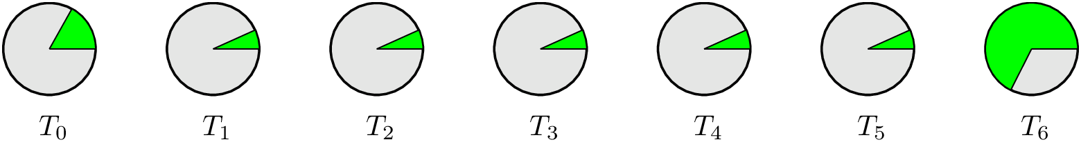
Ok, now we understand the initial setup, and we know our priors. Let’s start gathering evidence and using Bayes’ Theorem to update the probabilities we assign to the different theories.

First evidence, $e_1$: we roll a 6

Alright, let’s start. We roll… a 6. That is $e_1$. How does $e_1$ update the probability we assign to each of our seven theories? Let’s calculate this.

First of all, notice that the denominator of Bayes’ Theorem is the same for all seven calculations, so let’s figure that out first. (Graphically, we represent this as the total green area.)

$$\begin{array}{lclcl} Pr(T_0) \times Pr(e_1 \ |\ T_0) & & \frac{1}{7}\ \times\ \frac{1}{6} & & \frac{1}{42} \\ +\ Pr(T_1) \times Pr(e_1 \ |\ T_1) & & +\ \frac{1}{7}\ \times\ \frac{1}{15} & & +\ \frac{1}{105} \\ +\ Pr(T_2) \times Pr(e_1 \ |\ T_2) & & +\ \frac{1}{7}\ \times\ \frac{1}{15} & & +\ \frac{1}{105} \\ +\ Pr(T_3) \times Pr(e_1 \ |\ T_3) & = & +\ \frac{1}{7}\ \times\ \frac{1}{15} & = & +\ \frac{1}{105} \\ +\ Pr(T_4) \times Pr(e_1 \ |\ T_4) & & +\ \frac{1}{7}\ \times\ \frac{1}{15} & & +\ \frac{1}{105} \\ +\ Pr(T_5) \times Pr(e_1 \ |\ T_5) & & +\ \frac{1}{7}\ \times\ \frac{1}{15} & & +\ \frac{1}{105} \\ +\ Pr(T_6) \times Pr(e_1 \ |\ T_6) & & +\ \frac{1}{7}\ \times\ \frac{2}{3} & & +\ \frac{2}{21} \end{array} = 0.1667$$

Now let’s plug in the values for $Pr(T_n)$ and $Pr(e_1\ |\ T_n)$ for each of our theories, to get values for $Pr(T_i\ |\ e_1)$:

$$Pr(T_0 \ |\ e_1) = \frac{Pr(T_0) \times Pr(e_1 \ |\ T_0)}{0.1667} = \frac{1/7 \times 1/6}{0.1667} = 0.1428 = 1/7$$

Rolling a 6 didn’t change $T_0$’s probability at all! That makes sense, when you think about it: just one throw does nothing either to support, or to undermine, the theory that the die is fair. What about the other theories? Let’s see what it does to $T_6,$ the theory that the die is $\frac{2}{3}$ biased towards 6.

$$Pr(T_6 \ |\ e_1) = \frac{Pr(T_6) \times Pr(e_1 \ |\ T_6)}{0.1667} = \frac{\frac{1}{7} \times \frac{2}{3}}{0.1667} = 0.5713$$

0.5713 is much greater than 1/7, so our rolling a 6 has greatly increased the probability of the theory that the die is biased towards 6.

So, if rolling a 6 leaves the probability of $T_0$ alone, and greatly increases that of $T_6,$ where is the increase coming from? (It has to come from somewhere, because our theories are exhaustive and mutually exclusive.) It’s coming from the other bias theories. Rolling a 6 greatly decreases the probabilities that each of those is true. Let’s do $T_4$—the others are the same.

$$Pr(T_4 \ |\ e_1) = \frac{Pr(T_4) \times Pr(e_1 \ |\ T_4)}{0.1667} = \frac{\frac{1}{7} \times \frac{1}{15}}{0.1667} = 0.0571$$

This is much less than the probability that $T_4$ had initially.

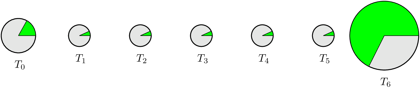
Here’s how the probabilities look graphically after we’ve acquired that first piece of evidence and used Bayes’ Theorem to update our estimates of the probability of each theory. Notice that while each theory has the same portion of green that it had before (which represents the conditional probability that 6 is thrown, on that theory), their sizes have changed to reflect the calculations we did of their post-$e_1$ probabilities.

Second evidence, $e_2$: we roll a 6 again

OK, now we throw again, getting a 6 a second time! That’s $e_2$. We can now apply Bayes’ Theorem again, using the probabilities that we assigned to them after we evaluated them in light of $e_1$. What will the Theorem tell us to do? Will $T_0$ remain unchanged? Let’s end the suspense.

As before we’ll start by doing the denominator, because it’s the same for all seven theories.

$$\begin{array}{lclclcl} Pr(T_0) \times Pr(e_2 \ |\ T_0) & & 0.1428 \ \times\ \frac{1}{6} & & 0.0238 \\ +\ Pr(T_1) \times Pr(e_2 \ |\ T_1) & & +\ 0.0571 \ \times\ \frac{1}{15} & & +\ 0.0038 \\ +\ Pr(T_2) \times Pr(e_2 \ |\ T_2) & & +\ 0.0571 \ \times\ \frac{1}{15} & & +\ 0.0038 \\ +\ Pr(T_3) \times Pr(e_2 \ |\ T_3) & = & +\ 0.0571 \ \times\ \frac{1}{15} & = & +\ 0.0038 & = & 0.4240 \\ +\ Pr(T_4) \times Pr(e_2 \ |\ T_4) & & +\ 0.0571 \ \times\ \frac{1}{15} & & +\ 0.0038 \\ +\ Pr(T_5) \times Pr(e_2 \ |\ T_5) & & +\ 0.0571 \ \times\ \frac{1}{15} & & +\ 0.0038 \\ +\ Pr(T_6) \times Pr(e_2 \ |\ T_6) & & +\ 0.5718 \ \times\ \frac{2}{3} & & +\ 0.3812 \end{array}$$

Notice that the conditional probabilities are unchanged by the new evidence. That’s because the probabilities of the theories are changing, not what the theories say. But this denominator—representing $Pr(e_2)$—is higher than before: the changes that we did in response to $e_1$ had that effect.

Now let’s plug in our values to get the probabilities we should assign to the theories after our second piece of evidence.

$$Pr(T_0 \ |\ e_2) = \frac{Pr(T_0) \times Pr(e_2 \ |\ T_0)}{0.4240} = \frac{0.0238}{0.4240} = 0.0561$$

So the second roll of a 6, unlike the first, does affect the probability that the die is fair. It reduces it from 0.1429 to 0.0561. A big drop.

$$Pr(T_6 \ |\ e_2) = \frac{Pr(T_6) \times Pr(e_2 \ |\ T_6)}{0.4240} = \frac{0.3812}{0.4240} = 0.8991$$

A big increase! And the probabilities of the other bias theories continue their declines; again let’s use $T_4$ as our representative:

$$Pr(T_4 \ |\ e_2) = \frac{Pr(T_4) \times Pr(e_2 \ |\ T_4)}{0.4240} = \frac{0.0038}{0.4240} = 0.0090$$

Here’s how this looks:

This is dramatically different both from the first and second distribution of probabilities. That’s the power of the Theorem: it shows up much more in its repeated application than in one-off applications.